
How I Made a Virtual Car Drive Itself, Part 3: Avoiding Collisions
| Timeline: | 2016-2018 | |
| Languages Used: | Python, C++, TensorFlow, Keras, OpenCV | |
| School: | Udacity, Colorado College | |
| Course: | Self-Driving Car Engineer Nanodegree |
How we got here: Sharing my Nanodegree Journey
Missed the previous posts in this series? No worries! Read the introduction to Terms 1 and 2:
…or read on to skip ahead! It’s your life, do what you want.
What’s next: Term 3
Now buckle your seatbelts as we dive into the challenging projects from the third and final term! In Term 3, I learned a more advanced algorithm for detecting the road even when objects are blocking the car’s view, and how to predict and plan out a path for the car’s future, instead of just reacting to current conditions.
1. Semantic Segmentation (Python/TensorFlow)
The semantic segmentation project uses a Fully Convolutional Network (FCN) to label each pixel in an image as “road” or “not road.” This is where the magic of deep learning gets visual.
Core Idea
The goal isn’t just to classify an image, like we were doing with traffic signs in Term 1, but rather to understand its content at a granular level. A truly autonomous car must understand its environment at a pixel level and be able to identify drivable space, even when there are obstructions.
The architecture is an FCN-8, a network famous for this kind of task, built on top of a pre-trained VGG16 model. A key tip from the project documentation was that the provided VGG model wasn’t vanilla; it was already a “fully convolutional version,” meaning its dense final layers had been swapped for 1x1 convolutions. This was a huge head start, as it meant I could directly tap into the rich feature maps from deep within the network.
The core of my implementation was the layers function, which reconstructs the final output by upsampling and combining layers from VGG. This is where the skip connections come in, merging the coarse, semantic information from deep layers with the fine, spatial information from shallower ones.
 1## main.py
 2def layers(vgg_layer3_out, vgg_layer4_out, vgg_layer7_out, num_classes):
 3    """
 4    Create the layers for a fully convolutional network.  Build skip-layers using the vgg layers.
 5    """
 6    # 1x1 convolution of vgg layer 7
 7    conv_7 = tf.layers.conv2d(vgg_layer7_out, num_classes, 1, strides=(1,1),
 8                                padding='same', kernel_regularizer=tf.contrib.layers.l2_regularizer(1e-3))
 9    # Upsample layer 7 output
10    output_7 = tf.layers.conv2d_transpose(conv_7, num_classes, 4, strides=(2,2),
11                                            padding='same')
12
13    # 1x1 convolution of vgg layer 4
14    conv_4 = tf.layers.conv2d(vgg_layer4_out, num_classes, 1, strides=(1,1),
15                                padding='same', kernel_regularizer=tf.contrib.layers.l2_regularizer(1e-3))
16    # Skip connection: add upsampled layer 7 to layer 4
17    skip_4 = tf.add(output_7, conv_4)
18    # Upsample the combined layer
19    output_4 = tf.layers.conv2d_transpose(skip_4, num_classes, 4, strides=(2,2),
20                                            padding='same')
21
22    # 1x1 convolution of vgg layer 3
23    conv_3 = tf.layers.conv2d(vgg_layer3_out, num_classes, 1, strides=(1,1),
24                                padding='same', kernel_regularizer=tf.contrib.layers.l2_regularizer(1e-3))
25    # Skip connection: add upsampled layer 4 to layer 3
26    skip_3 = tf.add(output_4, conv_3)
27    # Final upsample to restore original image size
28    output_3 = tf.layers.conv2d_transpose(skip_3, num_classes, 16, strides=(8,8),
29                                            padding='same')
30
31    return output_3
I trained the network on the KITTI Road dataset for 50 epochs with a batch size of 5. One of the trickiest parts was getting the L2 regularization right.
Tip
Udacity’s project instructions had a crucial tip: simply adding
kernel_regularizerto thetf.layerscalls isn’t enough in TensorFlow 1.x. You have to manually fetch the regularization losses and add them to your main cross-entropy loss function. It’s a classic “gotcha” that could easily go unnoticed.
The final model, trained with an Adam optimizer and a learning rate of 0.0008, produced some beautifully segmented images where the drivable area is highlighted.

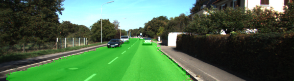
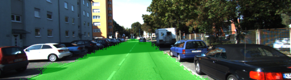
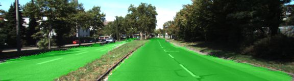
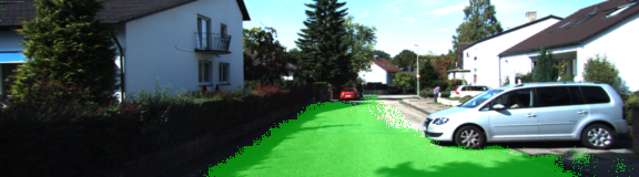
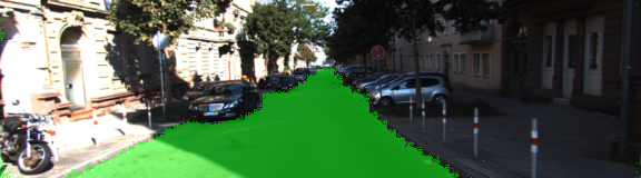
Fun fact: Seeing the model color in the road beneath the cars is weirdly satisfying.
2. Path Planning (C++)
The path planning project felt like the final exam, bringing together localization, prediction, and control into one C++ application. The goal was to build a “brain” that could safely navigate a busy highway, and the simulator didn’t pull any punches.
Core Idea
It’s not enough to just react to current conditions. Without predicting the future, avoiding a collision becomes an impossible task. The car must constantly observe the motion of other objects to plan safe paths and navigate complex roads in less than ideal conditions.
The challenge, as laid out in the project goals, was to make a car that drove politely but efficiently. It had to:
- Stay as close as possible to the 50 MPH speed limit.
- Automatically detect and overtake slower traffic by changing lanes.
- Avoid collisions at all costs.
- And crucially, do it all smoothly, without exceeding strict limits on acceleration and jerk. No one likes a jerky robot driver.
At every time step (every 0.02 seconds, to be exact!), the simulator fed my C++ program a stream of data: my car’s precise location and speed, and a sensor_fusion list detailing the position and velocity of every other car on my side of the road.
My code’s job was to act as a behavior planner using subsumption architecture. It would parse the sensor data to answer key questions:
- Is there a car directly ahead of me? If so, how far?
- Should I slow down to match its speed?
- Or, is the lane to my left or right clear for a pass?
Once the planner decided on an action (e.g., “prepare for a left lane change”), the next step was generating a smooth path. For this, I used a fantastic C++ spline library that was recommended in the project tips. It allowed me to take a few key waypoints, based on the car’s current state and its target destination, and interpolate a continuous trajectory for the car to follow.
1// Example: Find closest waypoint to start the path planning
2int ClosestWaypoint(double x, double y, const vector<double> &maps_x, const vector<double> &maps_y) {
3    // ... logic to find the nearest map waypoint ...
4    return closestWaypoint;
5}
 1// Using the spline library to generate the trajectory
 2#include "spline.h"
 3tk::spline s;
 4// Set anchor points for the spline based on current state and target
 5s.set_points(ptsx, ptsy);
 6
 7// Populate the next path points by evaluating the spline
 8vector<double> next_x_vals, next_y_vals;
 9for (int i = 0; i < 50; i++) {
10    // ... calculate points along the spline ...
11    next_x_vals.push_back(x_point);
12    next_y_vals.push_back(s(x_point));
13}
The beating heart of the project was a giant lambda function inside main.cpp: the h.onMessage handler. This function was called every 0.02 seconds with a fresh batch of telemetry data. This is where the magic happened: my code had to parse the car’s state, analyze the positions of all other cars on the road, and generate a safe and smooth trajectory, all in a fraction of a second.
Here’s a look at the structure of that handler, with pseudo-code outlining my decision-making logic:
 1// main.cpp
 2h.onMessage([&map_waypoints_x,...](uWS::WebSocket<uWS::SERVER> ws, char *data, size_t length, uWS::OpCode opCode) {
 3    // ... JSON parsing ...
 4    if (event == "telemetry") {
 5        // Get main car's localization data
 6        double car_x = j[1]["x"];
 7        double car_y = j[1]["y"];
 8        double car_s = j[1]["s"];
 9        double car_d = j[1]["d"];
10        double car_speed = j[1]["speed"];
11
12        // Get sensor fusion data: a list of all other cars
13        auto sensor_fusion = j[1]["sensor_fusion"];
14
15        // --- My Logic Started Here ---
16
17        // 1. Analyze the current situation using sensor_fusion data
18        bool car_ahead = false;
19        bool car_left = false;
20        bool car_right = false;
21        for (int i = 0; i < sensor_fusion.size(); i++) {
22            // Check if a car is in my lane, too close
23            // Check if cars are in the left/right lanes, blocking a change
24        }
25
26        // 2. Behavior Planning: Decide what to do
27        double target_speed = 49.5; // MPH
28        int target_lane = 1; // 0=left, 1=center, 2=right
29        if (car_ahead) {
30            if (!car_left) {
31                target_lane = 0; // Change to left lane
32            } else if (!car_right) {
33                target_lane = 2; // Change to right lane
34            } else {
35                target_speed -= .224; // Slow down to match car ahead
36            }
37        } else if (car_speed < 49.5) {
38            target_speed += .224; // Speed up to limit
39        }
40
41        // 3. Trajectory Generation using the spline library
42        // Create anchor points for the spline based on current state and target_lane/target_speed
43        // ... (as described in the spline example) ...
44        tk::spline s;
45        s.set_points(anchor_pts_x, anchor_pts_y);
46
47        // Populate next_x_vals and next_y_vals with points from the spline
48        // ...
49
50        // Send the new path back to the simulator
51        json msgJson;
52        msgJson["next_x"] = next_x_vals;
53        msgJson["next_y"] = next_y_vals;
54        auto msg = "42[\"control\","+ msgJson.dump()+"]";
55        ws.send(msg.data(), msg.length(), uWS::OpCode::TEXT);
56    }
57});
This approach of behavior planning combined with spline-based trajectory generation created a system that could navigate dynamic traffic safely and effectively. It was incredibly satisfying to watch my car make its own decisions to speed up, slow down, and weave through traffic to complete a full lap of the 6946-meter highway loop.
Reflections on the Nanodegree
I never got around to submitting my final project in Term 3, since I was too distracted by my new job in Google’s Engineering Residency. Udacity took a back seat while I prioritized converting onto my team as a FTE in Google Cloud, which I did successfully!
And I choose to believe the knowledge I took with me is far more valuable than any certificate.
Source Code
Ever taken on a project purely for the joy of learning? Let me know in the comments!