
How I Made a Virtual Car Drive Itself, Part 2: Taking Control in a Noisy World
| Timeline: | 2016-2018 | |
| Languages Used: | Python, C++, TensorFlow, Keras, OpenCV | |
| School: | Udacity, Colorado College | |
| Course: | Self-Driving Car Engineer Nanodegree |
How we got here: Sharing my Nanodegree Journey
Missed the first post in this series? No worries! Read the introduction:
…or skip ahead! It’s your life, do what you want:
What’s next: Term 2
Term 2 was exciting! In this term, we focused on algorithms for controlling the car based on real-world sensor data. Before getting into the fun details of PID and MPC, first we need to talk about filters!
1. Estimating the Car’s Position: Kalman Filters and Particle Filters
Core Idea
In robotics and autonomous vehicles, knowing exactly where you are is surprisingly hard. Sensors are noisy, the world is unpredictable, and GPS alone isn’t nearly accurate enough. That’s where estimation algorithms like Kalman filters and particle filters come in…
They combine noisy sensor data and a model of the system to estimate the true state of the vehicle (such as its position, velocity, and orientation) over time. Kalman filters are optimal for linear systems with Gaussian noise, while particle filters can handle highly nonlinear, non-Gaussian problems by representing the state as a set of random samples (particles).
Term 2 was where things got real. I implemented:
Extended Kalman Filter (EKF)
The EKF fuses noisy lidar and radar data to estimate a moving object’s state. The core update and prediction steps look like this:
 1// kalman_filter.cpp (EKF)
 2void KalmanFilter::Predict() {
 3    x_ = F_ * x_;
 4    MatrixXd Ft = F_.transpose();
 5    P_ = F_ * P_ * Ft + Q_;
 6}
 7
 8void KalmanFilter::Update(const VectorXd &z) {
 9    VectorXd z_pred = H_ * x_;
10    VectorXd y = z - z_pred;
11    MatrixXd Ht = H_.transpose();
12    MatrixXd S = H_ * P_ * Ht + R_;
13    MatrixXd Si = S.inverse();
14    MatrixXd PHt = P_ * Ht;
15    MatrixXd K = PHt * Si;
16
17    // new estimate
18    x_ = x_ + (K * y);
19    long x_size = x_.size();
20    MatrixXd I = MatrixXd::Identity(x_size, x_size);
21    P_ = (I - K * H_) * P_;
22}
For radar, the update step uses the nonlinear measurement function and its Jacobian:
 1void KalmanFilter::UpdateEKF(const VectorXd &z) {
 2    VectorXd h = tools.hFunction(x_);
 3    MatrixXd Hj = tools.CalculateJacobian(x_);
 4    VectorXd y = z - h;
 5    // normalize angle phi to [-pi, pi]
 6    // ... (angle normalization code)
 7    MatrixXd Ht = Hj.transpose();
 8    MatrixXd S = Hj * P_ * Ht + R_;
 9    MatrixXd Si = S.inverse();
10    MatrixXd PHt = P_ * Ht;
11    MatrixXd K = PHt * Si;
12
13    x_ = x_ + (K * y);
14    long x_size = x_.size();
15    MatrixXd I = MatrixXd::Identity(x_size, x_size);
16    P_ = (I - K * Hj) * P_;
17}
Reflection: Debugging the EKF was a crash course in linear algebra and sensor fusion. Getting the Jacobian and angle normalization right was tricky, but seeing the filter track a car’s position in real time was incredibly satisfying.
Unscented Kalman Filter (UKF)
The UKF handles nonlinearities better by propagating a set of sigma points through the process and measurement models:
1// ukf.cpp (UKF)
2void UKF::Prediction(double delta_t) {
3    SigmaPointPrediction(delta_t);
4    PredictMeanAndCovariance();
5}
Sigma points are generated and predicted as follows:
 1MatrixXd UKF::AugmentedSigmaPoints() {
 2    // create augmented mean vector, covariance, and sigma points
 3    // ...
 4    return Xsig_aug;
 5}
 6
 7void UKF::SigmaPointPrediction(double delta_t) {
 8    MatrixXd Xsig_aug = AugmentedSigmaPoints();
 9    // predict each sigma point
10    // ...
11}
The update step for radar uses the predicted sigma points to compute the mean and covariance of the predicted measurement, then updates the state:
1void UKF::UpdateRadar(MeasurementPackage measurement_pack) {
2    // PredictRadarMeasurement, then UpdateState
3}
Reflection: The UKF felt like magic! No more linearization headaches, just a cloud of sigma points smoothly tracking the car. But tuning all those noise parameters and weights was a delicate balancing act.
Particle Filter
For the “kidnapped vehicle” project, I implemented a 2D particle filter in C++. The filter maintains a set of particles, each representing a possible state. At each step, it predicts, updates weights based on sensor observations, and resamples:
 1// particle_filter.cpp (core methods)
 2void ParticleFilter::init(double x, double y, double theta, double std[]) {
 3    // Initialize particles with Gaussian noise
 4}
 5
 6void ParticleFilter::prediction(double delta_t, double std_pos[], double velocity, double yaw_rate) {
 7    // Predict new state for each particle
 8}
 9
10void ParticleFilter::updateWeights(double sensor_range, double std_landmark[],
11                const std::vector<LandmarkObs> &observations, const Map &map_landmarks) {
12    // Update weights using multivariate Gaussian
13}
14
15void ParticleFilter::resample() {
16    // Resample particles with probability proportional to their weight
17}
Reflection: The particle filter was both conceptually simple and surprisingly powerful. Watching the “cloud” of particles converge on the true position was a great visual for how probabilistic localization works. The biggest challenge was making the filter robust to noisy data and ensuring it ran fast enough for real-time use.
Summary: Implementing these filters gave me a deep appreciation for estimation theory. Each approach (EKF, UKF, and particle filter) has its strengths and quirks, but all share the same goal: making sense of a noisy, uncertain world.
2. PID Controller: My First Taste of Control
Core Idea
Controlling a car means more than just knowing where you are. You need to keep the car on track. PID controllers are a classic way to minimize errors and keep the vehicle centered and stable.
This project made the math of PID finally “click” for me. Here’s what I learned:
- P (Proportional): Controls how aggressively the car reacts to being off-center. Too high and the car wobbles; too low and it’s sluggish.
- I (Integral): Only useful if there’s a consistent bias (like a wheel misalignment). For this project, I set it to zero.
- D (Derivative): Smooths out the reaction, making steering more stable. Too low and the car oscillates; too high and it becomes unresponsive.
I manually tuned the parameters by trial and error in the simulator, aiming for a balance between quick correction and smooth driving. My best values:
- Steering: P = -0.2, I = 0.0, D = -3.0
- Throttle: P = -0.6, I = 0.0, D = 1.0
1// PID update (PID.cpp)
2double diff_cte = cte - prev_cte;
3int_cte += cte;
4double steer = -Kp * cte - Kd * diff_cte - Ki * int_cte;
I also used a PID controller for throttle, targeting a constant speed. The result? The car slowed down for sharp turns and sped up on straights, almost like a cautious human driver. Watching the effects of each parameter in real time was both enlightening and oddly satisfying.
3. Model Predictive Control (MPC): The Big Leagues
Core Idea
For more advanced driving, the car must plan ahead, predicting its future path and optimizing control inputs. MPC enables this by solving an optimization problem at every step: predicting future states and optimizing control inputs over a time horizon. It’s like chess, but for cars.
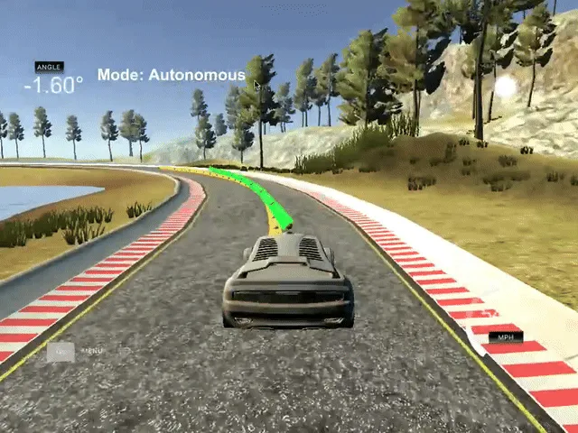
Note: In the simulation above, the yellow line represents the “ideal” trajectory at the center of the road, while the green line shows the car’s actual computed trajectory.
My MPC model followed the Udacity approach closely. The state vector included:
- x position
- y position
- steering angle (psi)
- velocity
- cross-track error
- orientation (psi) error
The actuators were steering and throttle. The cost function combined:
- cross-track error
- orientation error
- actuator changes (to penalize rapid steering/throttle changes)
I experimented with different prediction horizons and timestep lengths. After some trial and error, I settled on N = 10 and dt = 0.1 (so the prediction horizon T = 1 second). This was long enough for meaningful predictions but short enough for real-time computation. (Longer horizons were too slow; shorter ones didn’t give the car enough foresight.)
Before calling MPC.Solve(), I preprocess the waypoints by shifting the car’s reference frame to the origin and rotating it so the path ahead is horizontal. This makes polynomial fitting much simpler and more robust.
1// MPC cost function (MPC.cpp)
2for (int t = 0; t < N; t++) {
3    fg[0] += w_cte * CppAD::pow(cte[t], 2);
4    fg[0] += w_epsi * CppAD::pow(epsi[t], 2);
5    fg[0] += w_v * CppAD::pow(v[t] - ref_v, 2);
6}
One of the trickiest parts was handling latency. The simulator introduced a 100ms delay between sending actuator commands and seeing the result. To compensate, I simulated the car’s state forward by 100ms before running MPC, using the current steering and throttle values. This made the controller much more robust, almost as if there was no latency at all.
Reflection: The jump from PID to MPC felt like going from driving a go-kart to piloting a spaceship. Suddenly, I was thinking in terms of trajectories, constraints, and optimization. Tuning those hyperparameters was a balancing act between accuracy and computational cost, but when it worked, it felt like magic.
Source Code
Which algorithm do you prefer, PID or MPC? let me know in the comments!