
How I Made a Virtual Car Drive Itself, Part 1: Finding Lanes and Traffic Signs
| Timeline: | 2016-2018 | |
| Languages Used: | Python, C++, TensorFlow, Keras, OpenCV | |
| School: | Udacity, Colorado College | |
| Course: | Self-Driving Car Engineer Nanodegree |
Self-driven to Earn a Nanodegree
“You’re going to be one of our very first Self-Driving Car students!”
That was the subject line of the email I received from Udacity in 2016, and I still remember the jolt of excitement (and terror) that ran through me. Out of 11,000+ applicants, I was one of 250 accepted into the inaugural Self-Driving Car Engineer Nanodegree. The catch? I’d only driven a real car a handful of times.

I started Udacity’s online course while juggling my senior year at Colorado College, two thesis projects, and a job search that would eventually land me at Google.
The Nanodegree was a wild ride through computer vision, deep learning, estimation, and control. Here’s how I went from drawing lines on road images to unlocking the power of autonomous driving in a car simulator.
The Big Picture: Sharing my Nanodegree Journey
Already familiar with the topics in Term 1? Feel free to skip ahead to the more advanced algorithms:
1. Finding Lane Lines
Core Idea
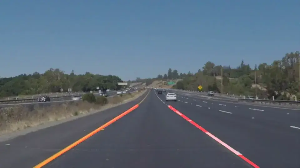
Before a car can drive itself, it needs to understand the road. The first step is detecting lane lines, which is crucial for keeping the vehicle safely in its lane and navigating turns.
Armed with OpenCV and a handful of image processing tricks, I built a pipeline that could find lines using color selection, Canny edge detection, and Hough transforms.

My results: Detecting a lane with a dashed white line on the left and solid white on the right

My results: Detecting a lane with a solid yellow line on the left and dashed white on the right
1## Lane detection pipeline (P1.ipynb)
2def pipeline(image):
3    gray = cv2.cvtColor(image, cv2.COLOR_RGB2GRAY)
4    blur = cv2.GaussianBlur(gray, (5, 5), 0)
5    edges = cv2.Canny(blur, 50, 150)
6    # ... region of interest, Hough transform, etc.
7    return result
The Hough Transform for Lane Detection
After edge detection, the Hough transform is used to find straight line segments that likely correspond to lane lines. The probabilistic Hough transform (cv2.HoughLinesP) maps edge points to a parameter space and finds the most likely lines by looking for intersections (votes) in this space.
 1def hough_lines(img, rho, theta, threshold, min_line_len, max_line_gap):
 2    """
 3    img should be the output of a Canny transform.
 4    Returns an image with hough lines drawn.
 5    """
 6    lines = cv2.HoughLinesP(img, rho, theta, threshold, np.array([]),
 7                            minLineLength=min_line_len, maxLineGap=max_line_gap)
 8    line_img = np.zeros((img.shape[0], img.shape[1], 3), dtype=np.uint8)
 9    draw_lines(line_img, lines)
10    return line_img
11
12def draw_lines(img, lines, color=[255, 0, 0], thickness=2):
13    """
14    Draws lines on the image inplace.
15    """
16    for line in lines:
17        for x1, y1, x2, y2 in line:
18            cv2.line(img, (x1, y1), (x2, y2), color, thickness)
Typical parameters:
1rho = 1            # distance resolution in pixels
2theta = np.pi/180  # angular resolution in radians
3threshold = 10     # minimum number of votes (intersections in Hough grid cell)
4min_line_len = 20  # minimum length of a line (pixels)
5max_line_gap = 300 # maximum allowed gap between line segments to treat them as a single line
Usage in the pipeline:
1edges = cv2.Canny(blurred_img, 50, 150)
2line_img = hough_lines(edges, rho, theta, threshold, min_line_len, max_line_gap)
3result = weighted_img(line_img, original_img)
Advanced Lane Detection
Beyond this, creating a robust solution for advanced lane detection involved iteratively tuning the color and gradient thresholds to create a robust binary image, experimenting with different combinations until the lane lines were reliably detected under varying lighting and road conditions. Key improvements included applying erosion and dilation to the directional binary output to remove isolated noise pixels, and using a positional mask to focus only on the relevant road area.
Handling cases where the lane detection sanity check failed was another challenge: initially, failed detections would trigger a full-image search, but if that also failed, the algorithm would fall back to drawing the average of the past 10 successful frames, greatly reducing erratic lane line behavior. These steps, along with careful perspective transforms and polynomial fitting, made the pipeline much more robust and predictable, even when lane markings were faint, partially missing, or barely visible under shadows.
Reflection: At first, I grouped line segments by slope (left/right), averaged their positions, and extrapolated to the bottom of the frame. Later, I improved robustness by clustering points and fitting lines of best fit, and even filtered for yellow/white in HSV color space for challenging lighting.
2. Traffic Sign Recognition & Deep Learning
Next up: teaching a neural network to recognize traffic signs from the German Traffic Sign Dataset. This was not my first real foray into deep learning, but I still spent way too long tuning hyperparameters and staring at loss curves.


How the Classifier Works
- Data: The model is trained on 32x32 RGB images, each labeled with one of 43 possible traffic sign classes. The dataset is diverse, with thousands of images per class, and includes real-world variations in lighting, angle, and occlusion.
- Preprocessing: Images are normalized to the range [0.1, 0.9] for better convergence. I also shuffled the data before each epoch to help the model generalize.
- Architecture: The network is a custom convolutional neural network (CNN) inspired by LeNet, but deeper and adapted for color images and more classes. It uses three convolutional layers, each followed by ReLU activations and max pooling, then flattens and passes through two dense layers before the final softmax output.
Neural Network Architecture (TensorFlow)


graph src
 1---
 2config:
 3  theme: 'base'
 4  themeVariables:
 5    primaryColor: '#333'
 6    actorTextColor: '#fff'
 7    primaryTextColor: '#aaa'
 8    primaryBorderColor: '#aaa'
 9    lineColor: '#F8B229'
10---
11sequenceDiagram
12    participant I as Input
13    participant C1 as Conv1
14    participant P1 as Pool1
15    participant C2 as Conv2
16
17    Note right of I: 32x32x3 Image
18    I->>C1: Pass Tensor
19    Note right of C1: 5x5 filters, 6 channels
20    C1->>P1: Pass Feature Map
21    Note right of P1: 2x2 Max Pooling
22    P1->>C2: Pass Feature Map
23    Note right of C2: 3x3 filters, 10 channels
 1---
 2config:
 3  theme: 'base'
 4  themeVariables:
 5    primaryColor: '#333'
 6    actorTextColor: '#fff'
 7    primaryTextColor: '#aaa'
 8    primaryBorderColor: '#aaa'
 9    lineColor: '#F8B229'
10---
11sequenceDiagram
12    participant C2 as Conv2
13    participant P2 as Pool2
14    participant C3 as Conv3
15    participant F as Flatten
16
17    Note right of C2: Input from previous stage
18    C2->>P2: Pass Feature Map
19    Note right of P2: 2x2 Max Pooling
20    P2->>C3: Pass Feature Map
21    Note right of C3: 3x3 filters, 16 channels
22    C3->>F: Pass Final Feature Map
23    Note right of F: Reshape to vector
 1---
 2config:
 3  theme: 'base'
 4  themeVariables:
 5    primaryColor: '#333'
 6    actorTextColor: '#fff'
 7    primaryTextColor: '#aaa'
 8    primaryBorderColor: '#aaa'
 9    lineColor: '#F8B229'
10---
11sequenceDiagram
12    participant F as Flatten
13    participant D1 as Dense1
14    participant D2 as Dense2
15    participant D3 as Dense3
16    participant O as Output
17
18    Note right of F: Input from previous stage
19    F->>D1: Pass Flattened Vector
20    Note right of D1: 120 units + ReLU
21    D1->>D2: Pass Vector
22    Note right of D2: 86 units + ReLU
23    D2->>D3: Pass Vector
24    Note right of D3: 43 units + Softmax
25    D3->>O: Pass Final Logits
26    Note right of O: Class Probabilities
 1## TrafficNet architecture (simplified)
 2def TrafficNet(x, dropout):
 3    # Layer 1: Conv2D, 5x5 kernel, 6 filters, ReLU
 4    c1 = conv2d(x, weights['wc1'], biases['bc1'], strides=1)
 5    # MaxPool 2x2
 6    p1 = maxpool2d(c1, k=2)
 7    # Layer 2: Conv2D, 3x3 kernel, 10 filters, ReLU
 8    c2 = conv2d(p1, weights['wc2'], biases['bc2'], strides=1)
 9    # MaxPool 2x2
10    p2 = maxpool2d(c2, k=2)
11    # Layer 3: Conv2D, 3x3 kernel, 16 filters, ReLU
12    c3 = conv2d(p2, weights['wc3'], biases['bc3'], strides=1)
13    # Flatten
14    flat = flatten(c3)
15    # Dense 120 + ReLU
16    fc1 = tf.nn.relu(tf.matmul(flat, weights['wd1']) + biases['bd1'])
17    # Dense 86 + ReLU
18    fc2 = tf.nn.relu(tf.matmul(fc1, weights['wd2']) + biases['bd2'])
19    # Output: Dense 43 (Softmax)
20    logits = tf.matmul(fc2, weights['wd3']) + biases['bd3']
21    return logits
Training & Results
- The model was trained using cross-entropy loss and dropout for regularization. I monitored validation accuracy after each epoch and tweaked the learning rate and dropout to avoid overfitting.
- After several rounds of tuning, the final model achieved high accuracy on the test set and could reliably classify real-world traffic sign images, even with noise and distortion.
Side note: Building and tuning this network gave me a much deeper appreciation for the power (and quirks) of deep learning. Watching the model go from random guesses to near-perfect accuracy was like watching a child learn to read, except the child is a bundle of matrix multiplications.
3. Behavioral Cloning: Teaching a Car to Drive Like Me
Core Idea
To automate driving, the car needs to learn how to steer based on what it “sees.” Behavioral cloning uses deep learning to mimic human driving by mapping camera images to steering commands.
I collected training data by manually driving laps in the Udacity simulator, focusing on center-lane driving, recovery from the sides, and even driving in reverse for robustness. Only the center camera images were used for simplicity.

My first behavioral cloning results: jerky driving and dangerous on corners
I experimented with different combinations of data: sometimes including recovery and reverse driving, sometimes just center lane, and even data from a second, more challenging track. Interestingly, the model trained only on center lane data performed best on the original track, while the more diverse data helped on the harder track but sometimes made the car less reliable on the first.
To augment the dataset, I flipped images and steering angles, effectively doubling the data and helping the model generalize:
1## Data augmentation: flipping images and angles
2def augment(sample):
3    image, angle = sample
4    flipped_image = cv2.flip(image, 1)
5    flipped_angle = -angle
6    return [(image, angle), (flipped_image, flipped_angle)]
A Python generator efficiently loaded and preprocessed images in batches, including shuffling and flipping:
 1## Data generator for efficient training
 2def generator(samples, batch_size=32):
 3    num_samples = len(samples)
 4    while True:
 5        shuffle(samples)
 6        for offset in range(0, num_samples, batch_size):
 7            batch_samples = samples[offset:offset+batch_size]
 8            images, angles = [], []
 9            for image, angle in batch_samples:
10                images.append(image)
11                angles.append(angle)
12            yield np.array(images), np.array(angles)
Cropping layers in the model removed irrelevant parts of the image (like the sky and car hood), and a dropout layer helped reduce overfitting. I used a validation split and found that training for just two epochs was optimal. More led to overfitting.
A fun (and frustrating) discovery: the simulator provided images in BGR format, but my model was trained on RGB. Fixing this bug in drive.py made a big difference:
1## Convert BGR to RGB before prediction
2display_image = cv2.cvtColor(image, cv2.COLOR_BGR2RGB)
The final model, based on the NVIDIA architecture, used several convolutional layers, RELU activations, max pooling, dropout, and dense layers:
 1model = Sequential()
 2model.add(Lambda(lambda x: x / 255.0 - 0.5, input_shape=(160,320,3)))
 3model.add(Cropping2D(cropping=((70,25), (0,0))))
 4model.add(Conv2D(24, (5, 5), activation='relu'))
 5model.add(MaxPooling2D((2, 2)))
 6model.add(Conv2D(36, (5, 5), activation='relu'))
 7model.add(MaxPooling2D((2, 2)))
 8model.add(Conv2D(48, (5, 5), activation='relu'))
 9model.add(MaxPooling2D((2, 2)))
10model.add(Conv2D(64, (3, 3), activation='relu'))
11model.add(Dropout(0.5))
12model.add(Flatten())
13model.add(Dense(100, activation='relu'))
14model.add(Dense(50, activation='relu'))
15model.add(Dense(10))
16model.add(Dense(1))
After much iteration, the best model could drive autonomously around the track without leaving the road (most of the time!).

My behavioral cloning results: The final iteration, with smoother driving
Source Code
How would you rate my driving for the cloning exercise? Let me know in the comments!